A5. MIS Foundational Elements Math

1) E = Energy Autonomy Foundation Calculation (MIS Lite)

Here is an example of the MIS Lite calculation used in the first century HE. Note: later periods significantly refined this approach using advanced scenario modelled monte carlo simulation probability but that is too complex to show here, but does not change the essence of the calculation.

a) Adequacy & Firmness (E_cap)

“Do we have enough firm power for critical load with headroom?”

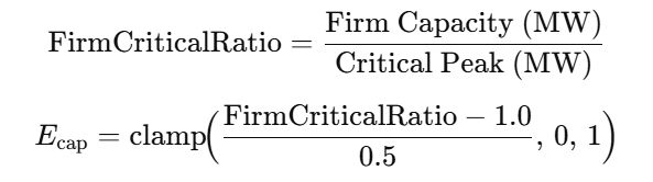
Count storage as firm up to 4 h at rated discharge.

Full score at +50% firm headroom (N-1/N-2 typically satisfied).

b) Flexibility via Storage (E_store)

“Can storage ride short/medium lulls without imports?” (multi-week belongs in S)

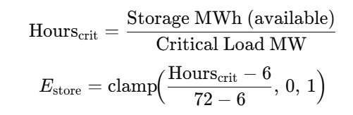
(6 h → 0; 72 h → 1; cap above 72 h.)

c) Diversity & Redundancy (E_mix)

“Are we fragile to one source?” Use Shannon evenness over delivered energy shares p_k​:

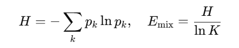
Tip: Use annual delivered energy shares, not nameplate.

d) Islanding & Sectionalization (E_island)

“How much critical load can run as independent micro-grids?”

f_islandable​: fraction of critical load on islandable circuits.

f_{islands-with-own-genf}​: fraction of critical load that sits on islands each with ≥2 sources (e.g., PV+CHP).

e) Black-start Readiness (E_black)

Step score by proven drills (take highest met):

0.0 = none

0.3 = planned black-start (cold to nominal) pass

0.6 = surprise black-start pass

0.8 = surprise under adverse conditions (dust/winter)

1.0 = multi-island black-start + re-synchronization proven

f) Energy Input Sovereignty (E_supply)

“How dependent is energy on imported fuels/parts (distinct from A/M)?”

Weights w_j​ reflect criticality × mass of carriers.

Scope guard: Keep multi-week stockpiles in S, not here.

Inputs:

Load model: critical (must never drop), essential (short outages OK), flexible/interruptible. Peak (MW) and average (MW).

Generation stack: nameplate & firm contribution by type (nuclear, PV, wind, CHP/Sabatier heat, etc.).

Storage: energy (MWh) and power (MW), availability, round-trip.

Grid topology: islandable circuits, sectionalization, # of independent islands with local gen.

Black-start drills: timestamps, scope, pass/fail.

Supply sovereignty: local share of energy carriers (e.g., CH₄/O₂ ISRU), and repair/production of power electronics (inverters, rectifiers, transformers).

2) L = Life Support Foundation Calculation (MIS Lite)

Here is an example of the MIS Lite calculation used in the first century HE. Note: later periods significantly refined this approach using advanced scenario modelled monte carlo simulation probability but that is too complex to show here, but does not change the essence of the calculation. This version turns ops data into a 0–1 score without double-counting A (mass localization) or S (buffer days).

a) Atmosphere closure (L_air)

O₂_regen_share: O₂ produced by electrolysis/bioprocess vs total O₂ demand (avg over ≥180 days).

CO₂_utilization_share: captured CO₂ routed into Sabatier/biomass (not vented).

Stability: % time within cabin O₂/CO₂ setpoint bands (0.0 at 95%, 1.0 at 99.9%+; scale linearly).

b) Water closure (L_water)

Recovery%: recycled water / total water demand (cap at 1.0).
Quality: compliance rate across potable/technical specs (bio/chem/particulate); penalize chronic biofilm/fouling.

c) Food & bioprocess closure (L_food)

kcal_share: locally grown/fermented edible kcal / required kcal.
MSI: micronutrient sufficiency index (0–1) from diet audits (protein, essential fats, vitamins / minerals).

d) Waste→resource closure (L_waste)

Nutrient_recovery: N/P/K returned to ag systems / N/P/K in waste.
Material_recovery: useful outputs (e.g., process water, polymer monomers) / total waste mass.

e) Loop robustness & controllability (L_robust)

Step score by proven drills (take highest met):

0.0 none; 0.3 planned failure-injection (sensor/valve/pump) pass;

0.6 surprise failure-injection pass; 0.8 surprise under adverse conditions (dust/winter);

1.0 multi-fault, degraded-mode operation ≥72 h + manual override competency verified.

Inputs:

Air loop: O₂ generation share, CO₂ removal & utilization, cabin setpoint stability (% time in range).

Water loop: recovery %, potable/technical water quality compliance, fouling/clean-in-place stats.

Food/bioprocess: local edible kcal share, micronutrient sufficiency index (MSI), crop/bioreactor uptime.

Waste→resource: fraction of solids/liquids turned into inputs (nutrients, water, reagents).

Fault tolerance: failure-injection outcomes, isolation latency, manual override drills.

Scope guard: L measures regenerative / recirculatory performance.

Do not count stockpiles or days of autonomy here → that’s S.

Do not count “local extraction” (e.g., ISRU water) as closure → that’s credited under A.

3) A = Autarky Mass Fraction Foundation Calculation (MIS Lite)

Here is an example of the MIS Lite calculation used in the first century HE. Note: later periods significantly refined this approach using advanced scenario modelled monte carlo simulation probability but that is too complex to show here, but does not change the essence of the calculation. 

a) Weight each item (mass × importance)

For each chokelist item j:

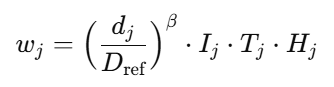
d_j​ : steady demand mass (kg per year or per HC).

D_ref​ : normalization (e.g., 10,000 kg).

Β ≈ 1 (keeps proportionality to mass burden).

I_j ∈ [0,1] : irreplaceability/criticality (oxygen, potable water, pressure hardware, steriles high; paint low).

T_j ∈ [0.4,1.0] : time-criticality/stockpilability (1.0 for non-stockpilable/short shelf-life; 0.7 for medium; 0.4 for long shelf-life).

H_j ∈ [0.8,1.2] (optional): hazard/safety multiplier for items whose loss is catastrophic (e.g., medical oxygen).

Publish your I / T / H tables once per rubric version.

b) Compute effective local share for each item

Start with the steady-state origin share:

Apply an origin factor (don’t over-credit assembly):

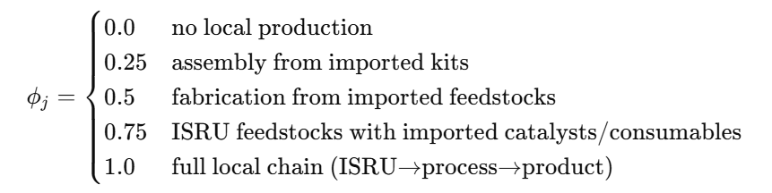
Apply quality compliance (spec + reliability):

Effective localization per item:

Notes:

If a functional substitute is used (e.g., polycarbonate panes replacing glass), credit it to the functional item group (publish your substitution map).

Use rolling 12-month (or 1 HC) evidence windows; count proven cadence, not one-off surges.

c) Aggregate to the pillar score

Weighted average across the chokelist:

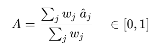
That’s it: A is “how much of the weighted, survival-critical bill of materials you truly supply from local origin at sustained cadence and acceptable quality.”

Inputs:

Chokelist v1.x items j with annual (or per-HC) demand mass d_j​ at required spec.

Local output time-series by item: measured mass meeting spec (not just nameplate) and steady-state cadence.

Origin & mode of production (assembly-only, fab from imported feedstock, full ISRU, etc.).

QA/acceptance: first-pass yield (FPY), field failure rates.

Weights metadata: criticality I_j​, stockpilability/time-criticality T_j​, optional hazard H_j​.

Scope guard:

A measures how much of the survival-critical bill you truly supply locally.

Don’t include days of stock (→ S) or ability to manufacture unrelated enabling kit (→ M).

Count only mass that originates locally (see “origin factor” below), not assembly of imported kits.

Common pitfalls & how to avoid them

Over-crediting assembly. Use the origin factor ϕ_j​ — assembly ≠ autarky.

Counting buffers here. Days of autonomy live under S, not A.

One-off hero runs. Score sustained cadence, not single shifts.

Hidden precursors. Catalysts/monomers/steriles are themselves chokelist items — account for them explicitly.

4) M = Manufacturity Breath Foundation Calculation (MIS Lite)

Here is an example of the MIS Lite calculation used in the first century HE. Note: later periods significantly refined this approach using advanced scenario modelled monte carlo simulation probability but that is too complex to show here, but does not change the essence of the calculation. 

a) Process coverage & depth (M_cov)

Use a standardized taxonomy (publish it with the audit). Score each process p as:

0.0 absent · 0.3 pilot/lab · 0.6 production single-line · 0.8 production with redundancy · 1.0 production + redundancy + validated interchangeability.

Suggested taxonomy (12 buckets; weight by foundational importance):

Foundations (heavier weight): mining/beneficiation; bulk metallurgy (Fe/Al); glass/ceramics; polymers/composites; cement/regolith.

Forming: casting/forging/extrusion/rolling; injection molding/thermoforming; additive manufacturing; glass forming.

Machining & joining: subtractive machining (CNC 3–5 axis); precision grinding/micro-machining; welding/brazing/adhesives & fastener standards; pressure-vessel fabrication.

Surface & heat-treat: heat treatment; coatings/finishes (PVD/CVD/plating/paint).

QA/metrology: dimensional (CMM/gage), materials lab, NDT (UT/RT).

Electronics (see M_elec for quality): PCB fab, SMT/PTH assembly, power-electronics assembly.

Compute:

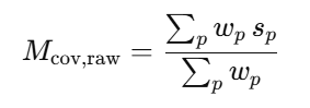
Apply a foundation penalty so missing bases bite:

(sˉ_foundations​ = weighted mean over foundations.)

b) Precision & properties maturity (M_tol)

“How tight and repeatable are you?”

TolScore: map the best routinely achieved ISO IT grade: IT12=0.2, IT10=0.4, IT8=0.6, IT7=0.8, IT6 or better=1.0 (use ≥200-part evidence).

FinishScore: map typical Ra: ≥3.2 µm=0.2, 1.6=0.4, 0.8=0.6, 0.4=0.8, 0.2=1.0.

PropertyControl: % batches hitting spec for hardness/strength/heat-treat ± tolerance (90%=0.6, 95%=0.8, 99%=1.0).

c) QA & metrology integrity (M_qa)

“Can you measure what you make—and swap parts at will?”

FPY: first-pass yield on top-20 parts (80%=0.6, 90%=0.8, 96%=1.0).

GageR&R: % of studies with %StudyVar ≤10% (70%=0.6, 85%=0.8, 95%=1.0).

Calibration: on-time rate for critical instruments (85%=0.6, 95%=0.8, 99%=1.0).

Interchangeability: blind swap tests pass rate for mating parts (80%=0.6, 90%=0.8, 98%=1.0).

d) Useful-node electronics capability (M_elec)

Ladder (take highest met, interpolate if mixed):

0.0 none

0.2 PCB assembly-only (imported boards)

0.4 PCB fab (1–2 layer) + SMT/PTH assembly + rework

0.6 4–6 layer PCB fab; ICT/flying-probe test; power-electronics assembly

0.8 sensor/packaging line (wire-bond/encapsulation) + conformal coat

1.0 discrete/power semis at relaxed geometries (e.g., >2 µm, HV MOSFET/IGBT/diodes) with redundancy

e) Uptime & reconfigurability (M_uptime)

“How reliably can cells run, and how fast can you pivot?”

OEE: average across critical cells (60%=0.4, 70%=0.6, 80%=0.8, 85%+=1.0).
PM: preventive maintenance schedule compliance (80%=0.6, 90%=0.8, 98%+=1.0).
SMED: median changeover time normalized to takt (0.6 for “half-shift”, 0.8 for “<2 hrs”, 1.0 for “<30 min”).

Inputs:

Process inventory: which processes you run in-hub at production grade (not just lab demos).

Status by process: absent / pilot / production (single-line) / production (redundant).

Precision & properties: routine tolerance classes, surface finish, heat-treat/property control.

QA & metrology: CMM/GD&T capability, materials lab, NDT, calibration compliance, interchangeability tests.

Electronics at “useful nodes”: PCB fab & assembly, sensor/packaging, discrete/power semis.

Uptime & reconfig: OEE, MTTR, preventive maintenance (PM) compliance, quick-changeover (SMED), cell redundancy.

Scope guard:

M = can we make the kinds of things survival demands?

Don’t count how much you make (that’s A), how long you can run (that’s S), or whether you can clone the whole base-kit (that’s R).

Common pitfalls & how to avoid them

Counting volume as breadth. Keep throughput in A; M is about capability coverage.

Over-crediting one hero CNC. Depth ≠ a single machine—ask for redundancy, QA, metrology.

Skipping electronics. Even limited “useful-node” capability massively reduces fragility.

Ignoring foundations. Penalize missing metallurgy/glass/polymers with the foundation factor.

Tooling drift. Without metrology & PM, capability decays—hence M_qa and M_uptime.

5) P = Population Viability Foundation Calculation (MIS Lite)

Here is an example of the MIS Lite calculation used in the first century HE. Note: later periods significantly refined this approach using advanced scenario modelled monte carlo simulation probability but that is too complex to show here, but does not change the essence of the calculation. 

a) Coverage & redundancy of critical posts (P_cov) — “Can we staff the system 24/7 with depth?”

For each role r:

(σ\sigmaσ = overhead for training/meetings; default 0.15.)

(Target backups per role default = 2 cross-qualified people.)

b) Training throughput & succession (P_pipe) — “Are replacements ready before people attrit?”

Two-deep fraction = roles with ≥2 qualified backups / total roles.

Throughput index = graduates to full-competence per year ÷ required replacements per year.

Refresh compliance = % of certs renewed on time.

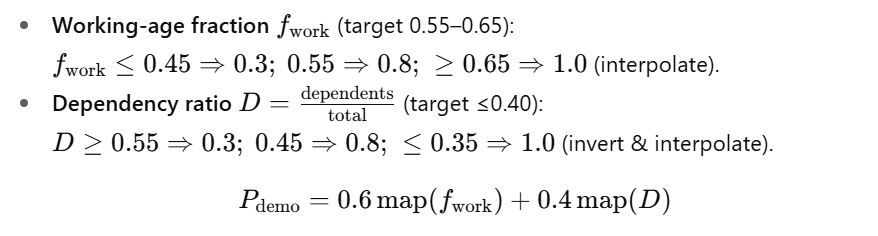
c) Demographic stability & dependency (P_demo) — “Is the age pyramid healthy?”

Map two observable ratios to 0–1:

d) Reproductive & genetic viability (P_rep) — “Can this population sustain healthy births for decades?”

Compute effective population size from current adults:

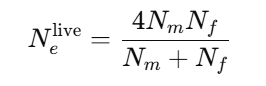
Add biobank equivalent (distinct, QC’d donor genomes):

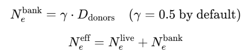
Map to 0–1 with survival-focused bounds:

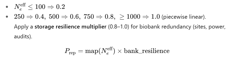
(Ethics & governance of donor use live in G; the capacity and diversity live here.)
Material_recovery: useful outputs (e.g., process water, polymer monomers) / total waste mass.

e) Healthcare baseline (non-epidemic) (P_health) — “Can we treat the routine and the urgent?”

ServiceBreadth: ED, ICU, surgery, OB, pediatrics, diagnostics (lab/rad), dialysis, mental health; 0.1 each present at production grade (+0.05 each if redundant).

Quality: normalize 3–5 metrics vs targets (e.g., time-to-surgery, post-op complication rate, perinatal outcomes).

Uptime: staffed-shift coverage for these services × equipment uptime (ventilators, anesthesia, imaging).

Keep outbreak containment capacity in B.

f) Fatigue, retention & psych resilience (P_fatigue) — “Will people last under HC isolation?”

Hours/RestCompliance: % staff within limits (e.g., ≤48 h/week) and EVA exposure caps.

CriticalRoleRetention: annual retention of top-critical roles (with backfills ready).

MH_access: utilization + time-to-appointment + confidentiality compliance.

Inputs:

Critical roles & posts: role list rrr, always-on posts per role, criticality weights w_r.

FTE availability: qualified people per role, shift model (e.g., 4.5 FTE/post to cover 24/7 + leave/training).

Backups & cross-skill matrix: # of cross-qualified backups per role; second operator depth.

Training pipeline: apprentices in flight, annual graduates, time-to-competence, certification refresh.

Demography: age structure, working-age fraction, dependency ratio (non-workers / total), births per year (or per HC).

Reproductive/Genetic assets: numbers of breeding-age Nm,Nf​, biobank donors (distinct sperm/egg/embryo genomes) and storage redundancy.

Healthcare baseline: service lines (ED/ICU/surgery/OB/peds/diagnostics), staff coverage, clinical quality and uptime.

Fatigue & retention: hours/rest compliance, role churn, EVA exposure limits, mental-health access.

Scope guards:

B handles outbreak detection/containment—keep epidemic drills out of P.

G holds documentation and policy quality; P cares whether people are trained, present, and replaceable.

S captures days of autonomy; don’t put stockpile days here.

Common pitfalls & how we avoided them:

Counting policy as capability. SOPs live in G; P wants staffed, qualified people.

Overlooking backups. One fully covered role with zero backups is still fragile.

Using stockpile days. Buffers are S, not P.

Ignoring biobank resilience. Donor count without redundant storage isn’t real.

Averaging away weak links. Weight critical roles higher in w_r​ so a single chokepoint drags P_cov (as it should).

6) R = Replication Capacity Foundation Calculation (MIS Lite)

Here is an example of the MIS Lite calculation used in the first century HE. Note: later periods significantly refined this approach using advanced scenario modelled monte carlo simulation probability but that is too complex to show here, but does not change the essence of the calculation. 

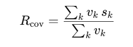
a) Base-Kit coverage (R_cov) — “Which modules can we rebuild locally to spec?”

For each module k with criticality weight vkv_kvk​ (publish once per version):

0.0 absent

0.3 assembly from imported kits

0.6 fabrication from imported feedstocks/jigs (production-grade)

0.8 largely local inputs; only commodity specials imported (e.g., catalysts)

1.0 full local chain (from local materials & in-hub processes) + passed acceptance tests

b) Recursion depth (R_rec) — “Tools that make the tools.”

Ladder (take highest met):

0.0 cannot reproduce any enabling tools

0.3 can duplicate plug-in modules (power, pumps) using installed machine shop

0.5 can reproduce first-line cells (life-support skid, pump/valve line) to spec

0.7 can reproduce machine-tool cell (castings→spindle/motion), and metrology cell (CMM/fixtures)

0.9 can reproduce electronics useful-node line (PCB fab + packaging + power discretes)

1.0 can reproduce the entire Base-Kit (Level-2 recursion) to spin up a new factory slice

c) Daughter-build proof (R_daughter) — “Evidence by replication.”

0.0 none

0.4 one Base-Kit module rebuilt & commissioned locally

0.6 three-module slice (e.g., power + machine-tool + metrology) built & run for 30 days

0.8 hublet (≥6 modules) built, integrated, and run for 60 days

1.0 hublet run under isolation for 90 days with documented ramp & maintenance

d) Toolchain sovereignty (R_sw) — “Can we rebuild our software stacks offline?”

0.0 vendor binaries only; cloud dependency

0.3 local mirrors of binaries; no rebuild

0.6 reproducible from source (CAD/CAM/EDA/PLC + compilers) in air-gap; signed builds

0.8 bootstrap compilers from trusted seeds; deterministic builds; SBOMs for all Base-Kit firmware

1.0 full toolchain bootstrapping from offline archives; periodic rebuild drills passed

e) Design & knowledge pack (R_docs) — “Everything you need to rebuild, version-controlled.”

Coverage: % of Base-Kit modules with CAD+BOP+test+maintenance packs (≥95% ⇒ 1.0).

Freshness: % updated in last 12 months / 1 HC (≥90% ⇒ 1.0).

Teach-back: pass rate on “build from docs only” drills.

f) Bio replication assets (R_bio) — “Can we reproduce biology-dependent starters & steriles?”

Ladder:

0.0 none

0.3 seed/strain bank only; no production

0.6 sterile disposables line + media prep + QC assays

0.8 vaccine/biologic starter capability (antigen or vector) + fill/finish

1.0 full bio Base-Kit: seed/strain + sterile + starter + QA with redundancy

g) Test & certification autonomy (R_test) — “Can we certify our own builds?”

Local_standards: hub-owned acceptance authority & procedures (pressure, electrical, bioprocess).

Calibration_chain: traceable to local primaries (mass/length/timebase/PNT).

Acceptance_rigs: % of Base-Kit modules with instrumented test rigs.

Inputs:

Base-Kit BOM v1.x: canonical module list k (e.g., power skid, life-support skid, pump/valve line, machine-tool cell, metrology cell, PCB+power-electronics cell, habitat pressure module, sterile manufacturing cell, ag/bioprocess module, sovereignty compute/PNT pack).

Build provenance per module: can it be built in-hub to spec? what external items are required? (bearings, cutting tools, catalysts, specialty ICs…).

Commissioning records: start-up, burn-in, test harness results.

Toolchain stack: CAD/CAM/EDA/PLC toolchains, compiler chain, package repos, signed builds.

Docs & knowledge pack: CAD, BOP (bill of process), test procedures, maintenance manuals, teach-backs.

Bio assets: seed/strain banks, starter cultures, reagent & sterile lines, QC assays.

Certification & metrology: local primary standards (mass/length/time), calibration chain, acceptance authority.

Scope guards:

Don’t count how much you can make (→ A).

Don’t count buffer days (→ S).

R credits capability to reproduce, proven by build + commission (not mock-ups).

7) S = Shock Isolation Resilience Foundation Calculation
(MIS Lite)

Here is an example of the MIS Lite calculation used in the first century HE. Note: later periods significantly refined this approach using advanced scenario modelled monte carlo simulation probability but that is too complex to show here, but does not change the essence of the calculation.

a) Isolation autonomy (multi-domain) — S_iso

For each critical item j, compute effective days:

Take a weighted median using w_j ∝ I_j^\*⋅T_j^\*​ (criticality × time-criticality from A-rubric). Normalize to the target horizon:

b) Achilles-heel balance — S_weak​

Penalize a single shortfall among top-weight items. Let D₅₀​ be the weighted median above and D_min​ the minimum D_j​ among the top-N weighted items (e.g., N=10).

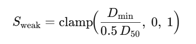
(=1.0 when the weakest key item is at least half the median; lower if there’s an Achilles heel.)

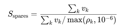
c) Spares depth for high-MTBF assemblies — S_spares

For each critical assembly k (pumps, valves, filters, power-electronics, ICU equipment, etc.), compute need over the horizon H = 780k days:

Effective supply = on-hand spares + local build capacity:

Coverage ratio ρ_k = min⁡(1, supply_k / need_k)

Aggregate with criticality weights v_k​ using a penalizing mean (harmonic):

d) Haven & route resilience — S_haven

f_cover​ : fraction of ops area within ≈100 km of a certified haven.

f_R≥2 ​: fraction of critical routes with ≥2 independent paths.

divert_score: map mean diversion time to [0,1] (e.g., ≥24 h ⇒ 0.2, 12 h ⇒ 0.6, ≤6 h ⇒ 1.0).

e) Continuity under import drought — S_ops

Ladder (highest met):

0.0 none

0.3 planned 30-day no-arrivals run (all critical services maintained)

0.5 surprise 30-day no-arrivals pass

0.8 surprise 60-day pass incl. constrained maintenance & load-shed to critical baseline

1.0 surprise 90-day pass with audited inventory telemetry & QA on deferred work

f) Cold-chain autonomy — S_cold

Let D_med and D_food be guaranteed days at spec temperature (with redundant power).

Inputs:

Isolation horizon target kkk in Hohmann Cycles (HC). Standard: k=10k{=}10k=10 for IL-6+ scoring. One HC ≈ 780 Earth days.

Critical consumables j: O₂, potable/process water, staple foods, fuels/heat, filters/membranes, medical steriles/PPE/reagents, power-electronics spares, bearings/seals, habitat spares, etc. For each: inventory Ij (with shelf-life), demand rate cjc_jcj​, criticality weights Ij\*,Tj\*​ (you can reuse the A-rubric weights), and substitution options.

Spares/failure data kkk: installed units, failure rates λk\lambda_kλk​, repair lead times, local build rates (if any), yield yk.

Mobility/haven network: refuge spacing, route redundancy, diversion times, inspection logs.

Continuity drills: “no-arrivals local-only” ops, import cutover tests, comms constraints if imposed.

Cold-chain telemetry: storage autonomy for temperature-critical meds/foods (redundant power included).

Scope guards:

S measures how long you can run with no physical inputs and how well you ride shocks.

Don’t count generation adequacy or black-start here (that’s E); don’t count new local production volumes (that’s A).

Keep outbreak drills in B; keep policies/SOPs quality in G.

Common pitfalls & how to avoid them

Hiding behind production. New local manufacturing is A; S asks “how long if nothing arrives.”

Counting black-start twice. Keep it in E; S uses no-arrivals continuity drills.

Mean-only autonomy. Use the weighted median and the Achilles-heel check to expose single points.

Ignoring shelf life & cold-chain. Autonomy days must be effective, not nominal.

Paper havens. Credit only inspected, stocked refuges on certified routes

8) G = Governance & Knowledge Foundation Calculation
(MIS Lite)

Here is an example of the MIS Lite calculation used in the first century HE. Note: later periods significantly refined this approach using advanced scenario modelled monte carlo simulation probability but that is too complex to show here, but does not change the essence of the calculation. 

a) Governance framework & crisis authority (G_org)

Ladder (take highest met):

0.0 ad-hoc leadership; no written triggers

0.3 charter + ICS documented; crisis triggers named; basic sunset clauses

0.6 tested crisis handover once; independent oversight body seated

0.8 dissimilar command paths (civil + technical); periodic reviews; public minutes

1.0 framework exercised under stress (brownout/comm limits) with post-action reforms enacted

b) Succession & handover readiness (G_succ)

For top-critical roles rrr: two-deep coverage and drill-proven handover.

c) Knowledge continuity (G_know)

Coverage, freshness, replication, and restorability of controlled documents.

Coverage: % of critical SOP/playbook/BOP sets present (target ≥95%).
Freshness: % updated within last 12 mo / 1 HC.
Replication: # independent replicas (≥2 sites, air-gapped) & WORM archives, normalized.
Restore: “bare-metal” restore & paper-mode procedure usability drill pass rate.

d) Auditability & transparency (G_audit)

Cadence: audits & drill reports released on schedule.

Closure: % audit findings closed within SLA.

Independence: ombuds red-team autonomy (budget, access) & public dissent logs.

e) Continuity under comms/coordination loss (G_cont). Ladder:

0.0 no drills

0.3 planned 48 h COG/COOP exercise, quorum maintained

0.5 surprise 72 h “dark-Earth” (signed, asynchronous, no live links)

0.8 surprise 14 d with degraded power/comms + lawful emergency acts & sunsets respected

1.0 surprise 30 d; decisions reproducible from signed logs; external oversight post-hoc

f) Scarcity procurement & substitution governance (G_proc)

TimeToAward: normalized median days from emergency trigger → award/issuance for critical SKUs.

SubstitutionCoverage: % chokelist items with pre-approved substitutions/specs.

Integrity: conflict-of-interest controls, dual-signatures, public spend ledger completeness.

Inputs:

Charter & crisis authority: written constitution/charter, incident command (ICS), crisis triggers, sunset clauses, emergency powers scope.

Succession & role coverage: top-critical roles list (e.g., 20–40), named successors, handover packs, cross-training.

Knowledge base: SOPs/playbooks/BOPs, version control (VCS), offline and replicated archives (WORM), restore drills.

Audit & transparency: public ledgers (chokelist stocks, drills), MIS change logs, red-team ombuds independence, audit cadence & closures.

Continuity drills: continuity-of-government (COG) / continuity-of-operations (COOP), dark-Earth (asynchronous, signed-only), quorum & decision logging.

Scarcity procurement & substitution: pre-approved suppliers, substitution rules, exception pathways, conflict-of-interest controls, time-to-award.

Scope guards:

Training throughput & staffing depth live in P; here we verify succession & handover fitness.

Outbreak response performance is B; here we score governance continuity during such events.

Stock levels are S; here we score rules and proof that decisions remain legitimate and documented.  

Common pitfalls & how to avoid them

Policies without practice. Require surprise drills and post-action reforms for top scores.

Docs online-only. Demand offline, replicated knowledge with periodic restore drills.

Leaders without backups. Score two-deep per critical role, not an average.

Opaque spending in emergencies. Tie awards to public ledgers and dual-signatures.

Conflating training with governance. Keep training throughput in P; G verifies the system stays legit and know-how survives.

9) B = Biosecurity & Epidemiology Foundation Calculation
(MIS Lite)

Here is an example of the MIS Lite calculation used in the first century HE. Note: later periods significantly refined this approach using advanced scenario modelled monte carlo simulation probability but that is too complex to show here, but does not change the essence of the calculation. 

a) Surveillance & Early Detection (B_surv)

Coverage: fraction of population/areas covered by wastewater + air + clinical sentinel sampling (≥80% ⇒ 1.0).

TAT: median time sample→actionable result (≤12 h ⇒ 1.0; 24 h ⇒ 0.8; 48 h ⇒ 0.6; >72 h ⇒ 0.3).

Genomic: share of positives sequenced (≥50% small outbreaks or ≥10% large ones ⇒ 1.0; map linearly).

b) Lab & Diagnostics Readiness (B_lab)

BSL_grade: BSL-2 present (0.4), BSL-3 access (0.7), local BSL-3 with redundancy (1.0).

Menu: fraction of required assay panel (respiratory, GI, bloodborne, fungal) validated in-hub.

Throughput: tests per day per 1k pop with TAT ≤24 h.

QC/PT: proficiency test pass rate, blind-sample accuracy.

c) Infection Prevention & Control Compliance (B_ipc)

AuditCompliance: observed compliance across PPE/hand hygiene/sterilization (≥95% ⇒ 1.0).

IsolationAdherence: % of indicated isolations/cohorting enacted within 2 h.

HAI_score: mapped inverse of healthcare-associated infection rates vs benchmarks.

d) Outbreak Containment Performance (B_resp)

Ladder (take highest met; real events trump drills; interpolate if mixed):

0.0 none; plans only

0.3 planned tabletop: complete contact chains; policies exercised

0.5 live exercise: contain to Rₜ<1 within 21 days; trace ≥80% contacts

0.8 surprise live drill under adverse conditions: Rₜ<1 in 14 days, isolation capacity not exceeded

1.0 real/sim event: Rₜ<1 in ≤7 days and cumulative incidence below target (e.g., <5/1,000), after-action reforms implemented

e) Clinical Isolation & Surge Capacity (B_iso)

AIIR_beds: negative-pressure or equivalent per 1k pop (target e.g., 0.5/1k ⇒ 1.0; map).

ICU/vent: staffed ICU beds & ventilators per 1k; uptime ≥0.95.

ACH_compliance: % isolation areas meeting airflow specs.

SurgeStaff: ability to double isolation capacity for ≥14 days (training rosters & drills).

f) Countermeasures Availability within Control Window (B_cmx)

CM_coverage: fraction of essential countermeasures ( vax / antivirals / antibiotics / diagnostics / PPE / fluids) with enough courses on-hand or callable to implement protocol within specified control windows (e.g., post-exposure prophylaxis ≤48 h). Do not score by “days of stock.”

Local_compounding: ability to compound/fill-finish steriles & prepare diagnostics locally to protocol specs within those windows (credit even if inputs arrive from A, as long as turnaround meets control targets).

Inputs:

Surveillance: wastewater/air/environmental sampling cadence & coverage; clinical testing volumes; time-to-result (TAT); genomic sequencing share of positives.

Laboratories: BSL-2/3 availability & redundancy; assay menu vs required panel; throughput & QC proficiency (EQA/PT).

IPC (infection prevention & control): audit compliance (hand hygiene, PPE, sterilization, cleaning), HAI rates, isolation protocol adherence.

Outbreak drills/events: time to index isolation, contact tracing coverage, time to Rₜ<1, case curves; tabletop vs live exercises; adverse-condition runs.

Clinical isolation & surge: negative-pressure/AIIR beds per 1k pop, cohorting options, ICU/vent support, ACH (air changes/hour) compliance, surge staffing.

Countermeasures readiness: vaccine program coverage & boosters; essential therapeutics/diagnostics/PPE on-formulary and available within control windows; local compounding/production capability for steriles/reagents.

Comms & consent artifacts: risk comms SOPs, public alerting, data dashboards (operational evidence only—policy quality is scored under G).

Scope guards:

No days-of-autonomy here (those live in S, including cold-chain autonomy).

Manufacturing volume credits live in A/M; B cares that countermeasures are available in time to control outbreaks.

Workforce staffing depth lives in P; here we verify epidemiology/IPC performance.

Common pitfalls & how to avoid them

Counting stockpile days. Keep autonomy days in S (use Scold for cold-chain); in B, score speed to deploy countermeasures.

All tabletop, no surprise drills. Reserve top scores for surprise or real events with fast Rₜ control.

Lab without throughput/QC. Validate assay menu + capacity + proficiency, not just a room with a sign.

IPC on paper. Measure adherence and HAI outcomes; audit regularly.

Single-path comms. Ensure outbreak ops work in dark-Earth/asynchronous modes (coordination quality in G, performance effect shows up in B_resp).

10) C = Social Cohesion & Alignment Foundation Calculation (MIS Lite)

Here is an example of the MIS Lite calculation used in the first century HE. Note: later periods significantly refined this approach using advanced scenario modelled monte carlo simulation probability but that is too complex to show here, but does not change the essence of the calculation.

a) Legitimacy & trust (C_trust) — Will people follow lawful direction under stress?

TrustIndex: average of 3 survey items (0–100): “trust ops leadership,” “fair process,” “willing to comply in emergency.” Map 60→0.6, 70→0.7, 80→0.85, 90→1.0 (clip at 0.3 minimum).

Participation: turnout at elections/assemblies or binding polls (≥70% ⇒ 1.0; 60% ⇒ 0.8; 50% ⇒ 0.6).

b) Fair allocation & grievance resolution (C_equity)

FairnessAudit: share of audited allocation queues (food/housing/EVA/training) meeting fairness criteria (≥95% pass ⇒ 1.0).

GrievanceClosure: % cases closed within SLA with feedback (≥90% ⇒ 1.0).

AppealQuality: independent reversals appropriately rare (U-shaped penalty); target reversal rate band 5–15% ⇒ 1.0.

c) Order, safety & discipline (C_order)

Use rates per 1k people, smoothed (e.g., Bayesian) to avoid volatility.

IncidentScore: inverse mapping of violent/sabotage/safety-critical violations to [0,1] vs benchmarks.

DrillCompliance: % residents meeting instructions in surprise drills within time windows.

WorkStability: strike/slowdown days and unauthorized absence, normalized (low is good).

d) Civic participation & mutual aid (C_civic)

MaintenanceRitual: attendance rate at weekly/monthly community maintenance (Sol-Six style).

VolunteerHours: hours per adult per quarter in community ops.

CrossTrainingUptake: % adults completing one new critical support skill per year.

e) Crisis communications hygiene (C_comms)

RumorTTD: median time-to-detect harmful rumor (≤2 h ⇒ 1.0; 6 h ⇒ 0.7; 12 h ⇒ 0.5).

CorrectionReach: share of residents receiving verified correction within target window (≥90% in 6–12 h ⇒ 1.0).

DarkEarthReady: comms delivery in signed/asynchronous modes (tested), multilingual support.

f) External alignment & de-escalation (C_ext) — Play nice, stay independent.

ChannelUptime: % availability of inter-hub diplomatic/ops channels.

JointDrills: cadence & pass rate of inter-hub drills (logistics aid, SAR, standards interop).
DeEscalation: proportion of cross-hub disputes settled within SLA without escalation.

Inputs:

Legitimacy & trust: periodic micro-surveys (institutional trust, perceived fairness, willingness to comply in emergencies), participation rates (elections/assemblies).

Equity & grievance: allocation fairness audits (food, housing, EVA slots, training seats), grievance intake & time-to-closure, appeals outcomes.

Order & discipline: safety/violence incidents per 1k people, strike/slowdown days, drill compliance breaches.

Civic participation: maintenance ritual attendance (e.g., Sol-Six), volunteer hours, cross-training uptake.

Crisis comms: rumor detection time, correction reach/latency, multilingual delivery, dark-Earth comms.

External posture: inter-hub treaties/MOUs, live comms uptime, joint drills, de-escalation outcomes, sanction-resilience exercises.

Scope guards:

G scores structures & records (charters, audits, succession). C scores lived adherence & social stability.

B scores outbreak performance. C may include general drill compliance, not epidemiology specifics.

P covers staffing & training throughput. C looks at participation and retention as civic behavior.

Common pitfalls & how to avoid them:

Politicizing the score. Keep to behavior-based, auditable proxies; publish methods; avoid identity metrics.

Survey bias & volatility. Use short, frequent micro-surveys with consistent wording; smooth with rolling medians; disclose N and error bars.

Counting paper protocols. Those live in G; C demands observed adherence and outcomes.

Single bad month spikes. Use smoothed rates and Bayesian shrinkage for small populations; add narrative context.

Opaque negative events. Require public, anonymized incident summaries and after-action remedies.